

Why RocksDB, Cassandra, and LevelDB Don’t Use B+ Trees
Comparing LSM Trees and B+ Trees Through Real-World Systems and Workload Patterns

When we think about indexes in a database, one common structure that comes to our mind is B+ trees. And it’s true!
They're the default in many relational databases like PostgreSQL and MySQL. They’re amazing for fast reads and efficient range scans.
But do you know that not all databases use B+ trees?
If we look at systems like RocksDB, Cassandra, or LevelDB, they’ve taken a completely different route with something called an LSM Tree (Log-Structured Merge Tree). And that choice isn’t random.
It all comes down to the kind of workload the system is designed for.
Disclaimer: This post will not be a deep dive into what B+ trees are; I am sure many posts explain B+ trees far better than I can.
This post will examine the differences between B+ trees and LSM trees, HOW they work, WHY they are needed, and HOW they make read/write operations efficient.
B+ Trees
Let’s recap the structure of B+ trees and how reads and writes happen —
Structure
In the below B+ tree, let’s assume there can only be at most 3 key nodes, or a maximum of 4 children for each node.
Read
We know the B+ trees are best for read-heavy systems. It performs really well in range queries, too.
Let’s understand why.
Equality Search
Let’s search for the key 15.
We should note that the actual keys are in the leaves; the other 15 that we see above the leaf are just the delimiters, to point us to the right subtree.
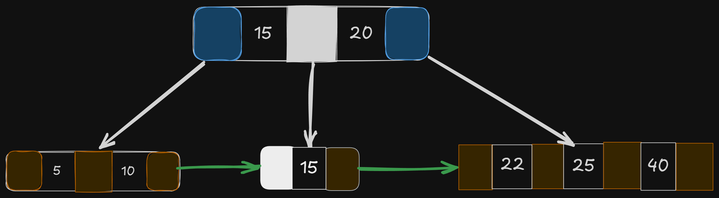
Just follow the white pointers, and you will reach 15.
Search happens in O(log(n)) or O(height of the tree).
Range Search
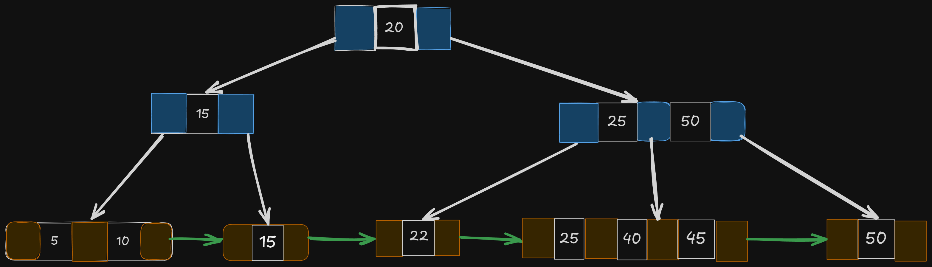
Let’s search for all the keys in the range [12, 38]
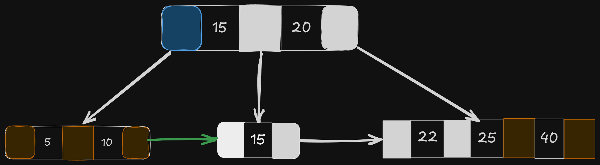
Notice the amazing feature of the B+ tree — the leaf nodes point to each other.
All we need to do is find the pointers >= 12 and <= 38, and we keep iterating from the start to the end pointer to get all the keys in that range.
This feature is pretty amazing, and when I found it for the first time, I was actually impressed.
Write
We know that indexing makes reads faster, but affects writes. Let’s understand what happens when a new key is added to a B+ tree, and why it slows down the writes.
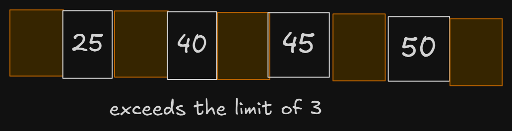
Let’s insert the key 45 in our tree —
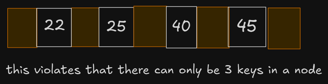
Since 45 comes after 40, it should get inserted in that order. But we see that our limit of 3 keys per node gets exceeded in this case.
This means we will have to split and rearrange the tree.
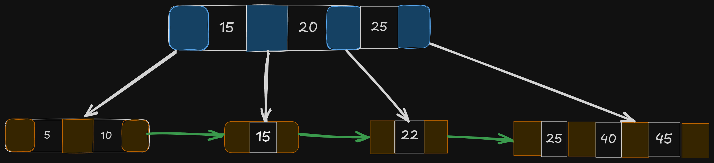
Get the middle key — 25
Copy the key, and move to its parent
Check if the parent has available slots (< 3); if so, insert the key as a delimiter and make it point to the next subtree
Inserting 45 wasn’t that expensive, since the parent has 1 available slot for the key to get inserted. What happens when even the parent is full?
Let’s insert 50 in the updated tree now —
Inserting 50 at its place exceeded the limit of that node, meaning the tree needed to be split and rearranged.
Let’s get the median, 40, and try putting it in its parent —
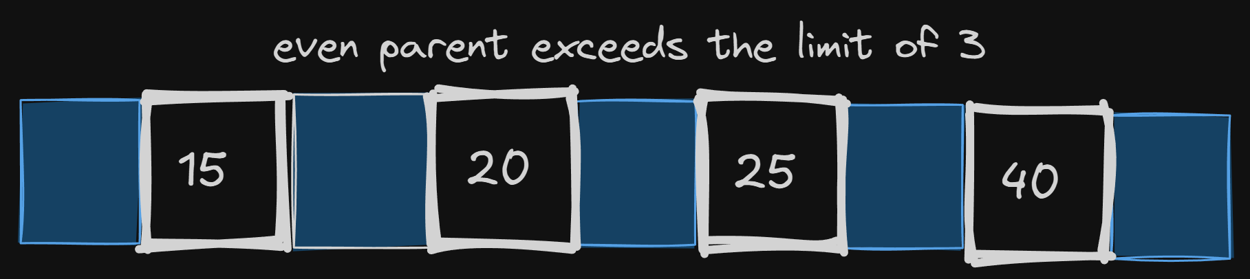
Even the parent is full now. And now we are at the root level, there is no parent now.
What do we do? We will do something similar we did when a node limit gets filled —
Pick the middle value (20)
Promote it to be the new root
Handle other values accordingly, as we did when inserting 45
So, from this insertion, we see that there can be changes not just at 1 level, but it can propagate till the root and restructure the whole tree, which is inefficient for write-heavy operations.
Storage
The above reason is why not all the nodes in B+ trees are filled all the time. It’s configured to be around 67% filled so that insertions are easier and we don’t have to rearrange the entire tree.
Imagine a tree with average fan out (no. of children from a node) = 133
Height 3 →
133^3 = 2,352,637 recordsHeight 4 →
133^4 = 312,900,700 records
You can see that even at a small height of trees, it can store millions of records, making it fast and efficient when it’s a read-heavy system.
But it is less efficient when there are frequent updates in the tree, resulting in many rearrangements.
LSM (Log-Structured Merge) Tree
For a write-heavy system, the structure of the LSM tree makes it much more efficient. Let’s understand the key components of an LSM tree.
Structure
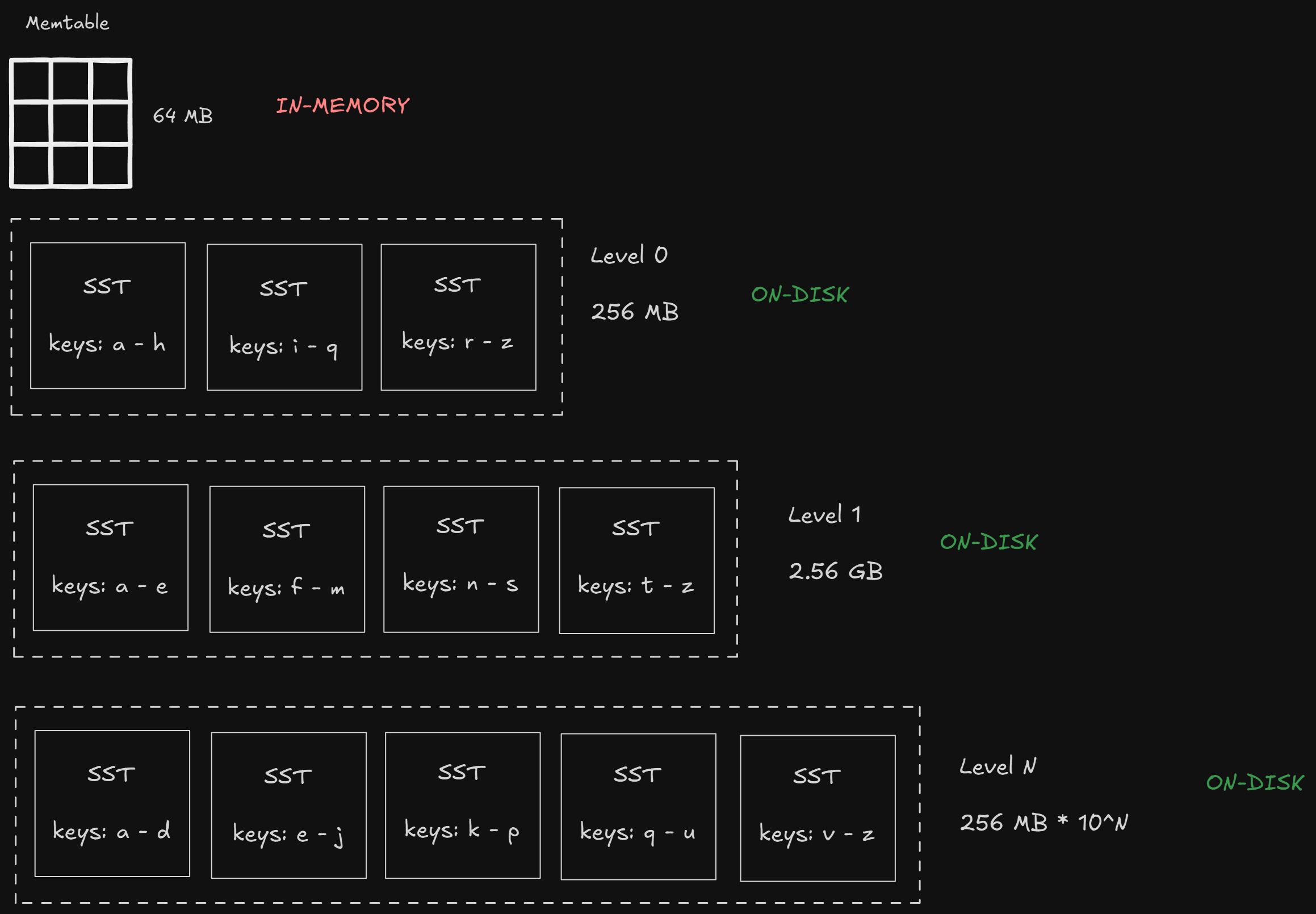
There are multiple different data structure that together makes the LSM tree —
At the top, there is a memtable, which contains the most recently inserted data; it is in-memory
As we go down, we get to different SST levels from 0 to N, each stored on disk
Each of the memtable and the lower levels has a subset of data at that level, incrementally in a sorted order
If any of the current levels are full, it is merged with the next level
This might feel overwhelming now, but let’s break down each of these components in more detail.
Memtable
This is the layer that is in-memory and has a fixed size. Once it exceeds its size, it’s converted into an immutable table, and it’s written to the disk in level 0.
It is an append-only data structure, implemented as "skip lists". For deletes, it just "marks" the key as deleted, instead of actually deleting it.
Skip List
Skip list is just like a linked list, but with multiple levels.
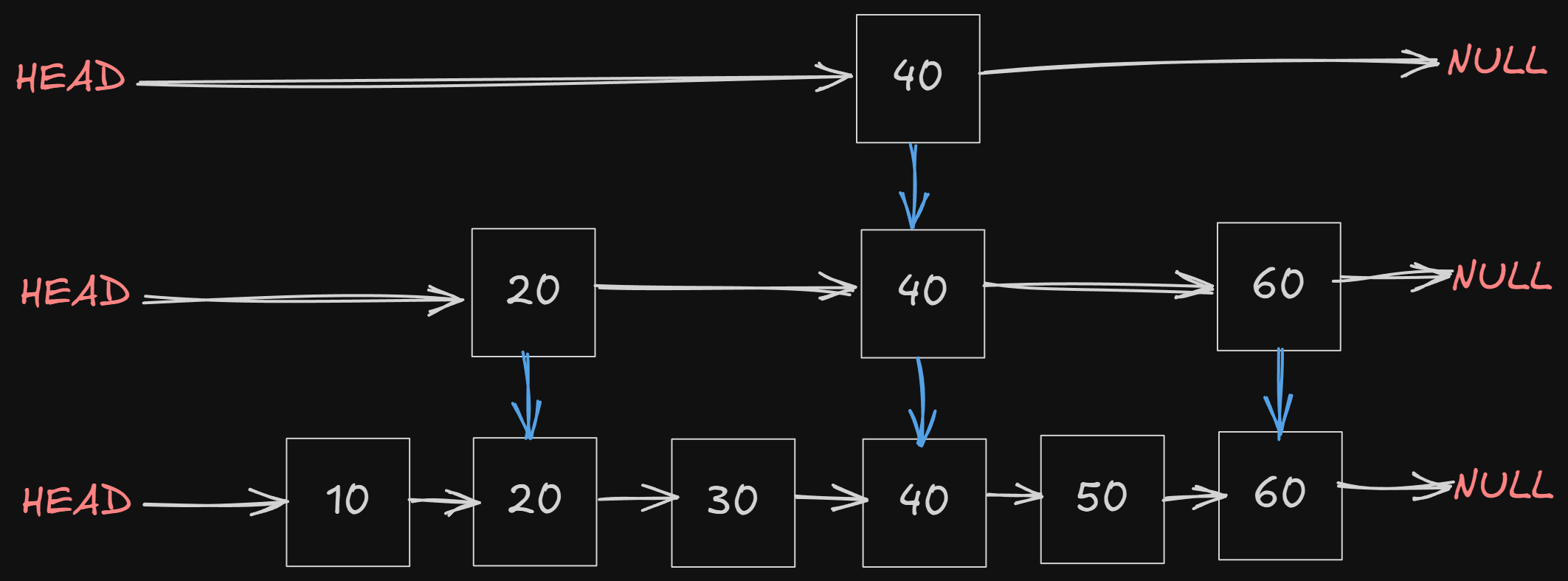
Some of the keys are promoted to different levels in a skip list. So when we search for a key, we might get that key before traversing the whole list. It’s random, but more efficient than traversing the whole list.
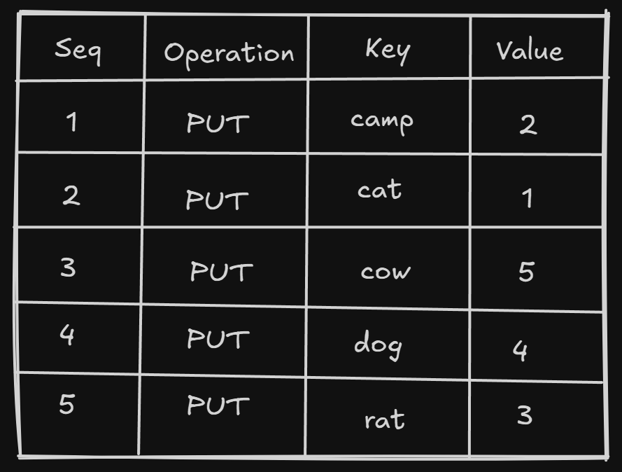
Let’s add some keys to the memtable —
db.put("cat", 1)
db.put("camp", 2)
db.put("rat", 3)
db.put("dog", 4)
db.put("cow", 5)
These keys will be stored in a sorted order, not in the order that they are inserted, so that it searches faster.
This will be the state of the memtable after inserting the above keys —
Write Ahead Log (WAL)
So we saw that memtable is completely in-memory. What happens if the application is restarted, or it crashes? We will lose things in memory.
To avoid this, the database writes all the updates to a WAL on disk.
So when the application restarts, it will replay those WALs and create the memtable.
WAL contains 4 things —
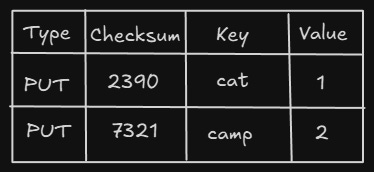
These are in order of updates, not sorted, so it can replay these in order.
Flush
When the memtable becomes full, it is converted into an immutable memtable, and the database runs a thread that writes the immutable tables to Level 0 on disk.
SST (Static Sorted Table)
The different levels are in the form of an SST (static sorted table). It has different blocks of a fixed size, and the data is organized in blocks in sorted order. These blocks can be compressed further with compression algorithms.
It has multiple sections -
Data section - contains the actual data, in an ordered manner
Index section - it contains the key and the offset of the block in which they reside; it is also sorted, so we can perform a binary search
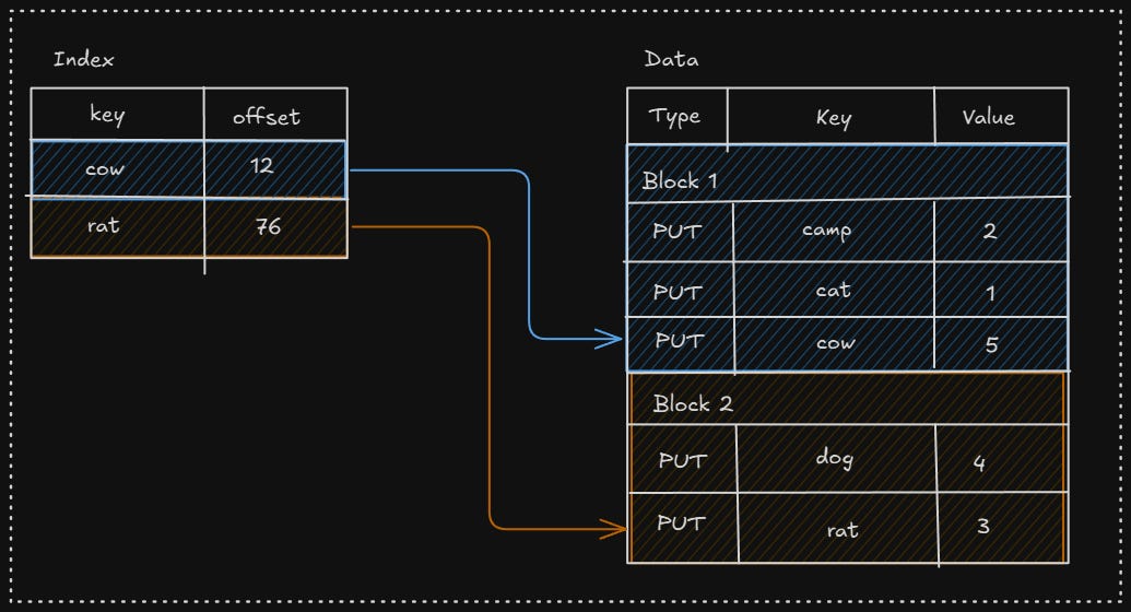
Let's say we search for "lynx", we will see that it might reside in block 2.
We will search block 2, but "lynx" is not there. It also provides bloom filters, that is used to test if an element belongs to a set or not.
A Bloom filter is a space-efficient probabilistic data structure used to quickly check whether a key might exist in a set.
Compaction
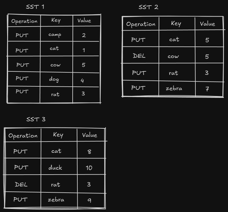
As the no. of writes increases, the memtable and different levels get filled fast. Because each put/delete operation is appended, there are many redundant forms of a single key. Consider the following operations —
db.delete("cow")
db.put("cat", 5)
db.put("rat", 3)
db.put("zebra", 7)

// Flush triggers
db.delete("rat")
db.put("cat", 8)
db.put("zebra", 9)
db.put("duck", 10)
This is the state of the SST after the above operations —
The space taken by deleted keys or updated keys is never reclaimed.
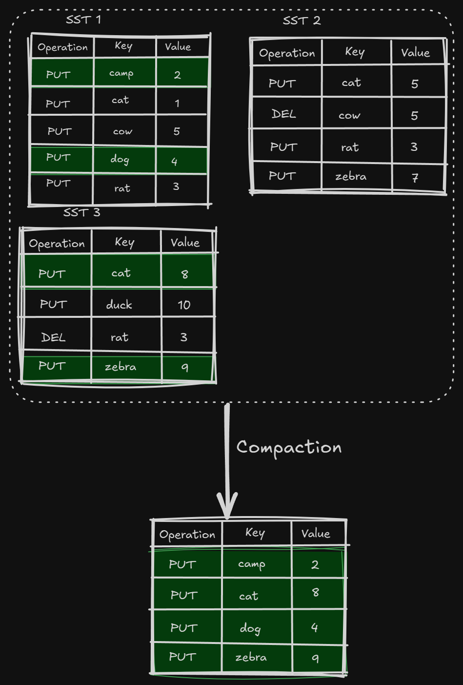
Reads get slower, as if we want to get a key, we need to search through all these SSTs to get the correct value. That's where compaction comes in.
Compaction helps to reduce space and read amplification in exchange for increased write amplification.
Compaction selects SST files on one level and merges them with SST files on a level below, discarding deleted and overwritten keys. Compactions run in the background on a dedicated thread pool, which allows the database to continue processing read and write requests while compactions are taking place.
Space amplification measures the ratio of storage space to the size of the logical data stored. Let's say, if a database needs 2MB of disk space to store key-value pairs that take 1MB, the space amplification is 2.
Read amplification measures the number of IO operations to perform a logical read operation.
We only take the updated values for the keys and discard all the deleted keys.
A L0 and L1 compaction can cascade to Level N. They are merged with the k-merge algorithm, similar to merge sort.
Now that we know all the components of an LSM tree, let’s understand the read and write paths.
Write Path
LSM tree is said to be efficient for write-heavy workloads. Let’s understand what happens for a write, step by step —
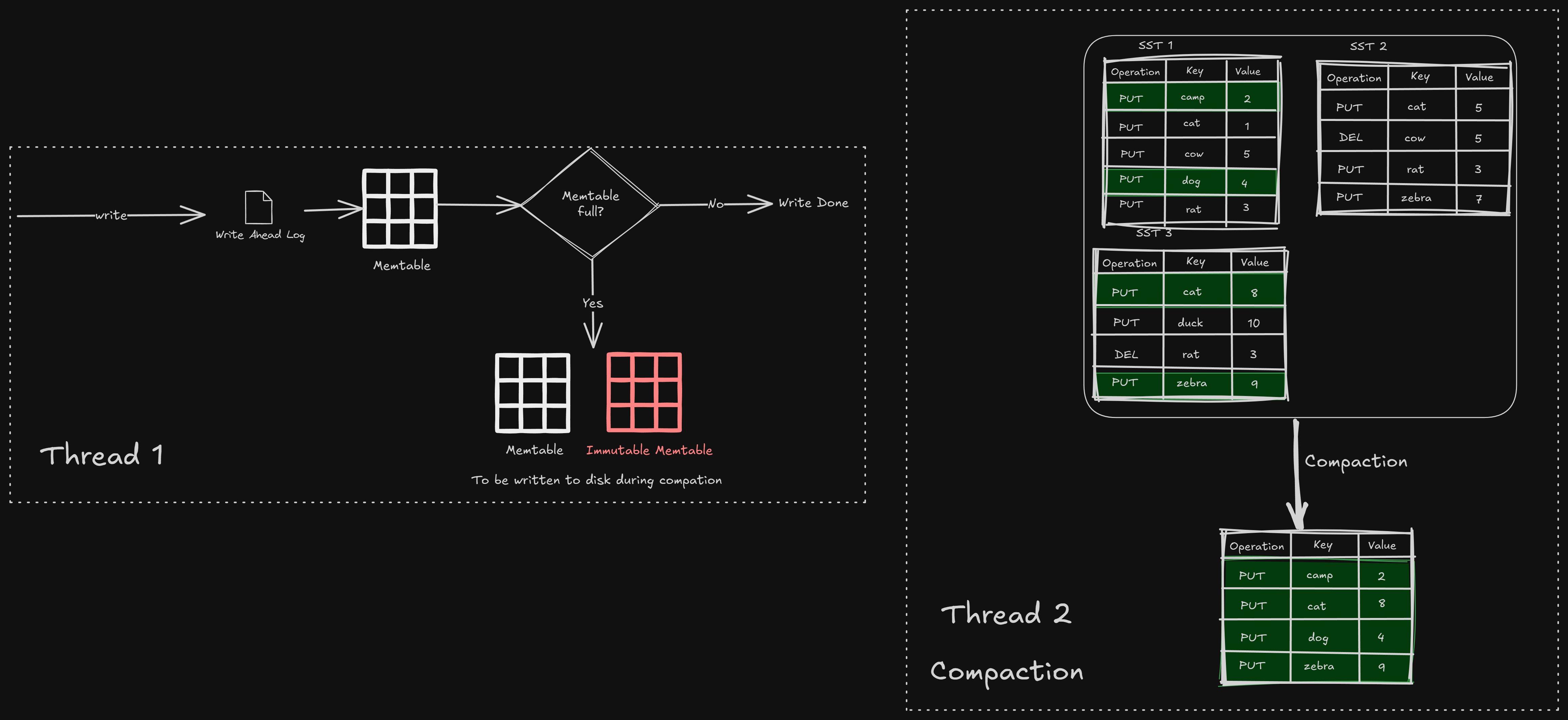
Every new write is first written to a WAL
It checks if the current memtable has space, it writes to it, otherwise creates a new memtable and marks the older one as immutable, to be written to disk in the next compaction/flush
That’s it! This is why it is fast, because all the compaction and flushing happen on a separate thread, making it write-heavy.
Read Path
Let’s understand what all things happen when we want to read a key —
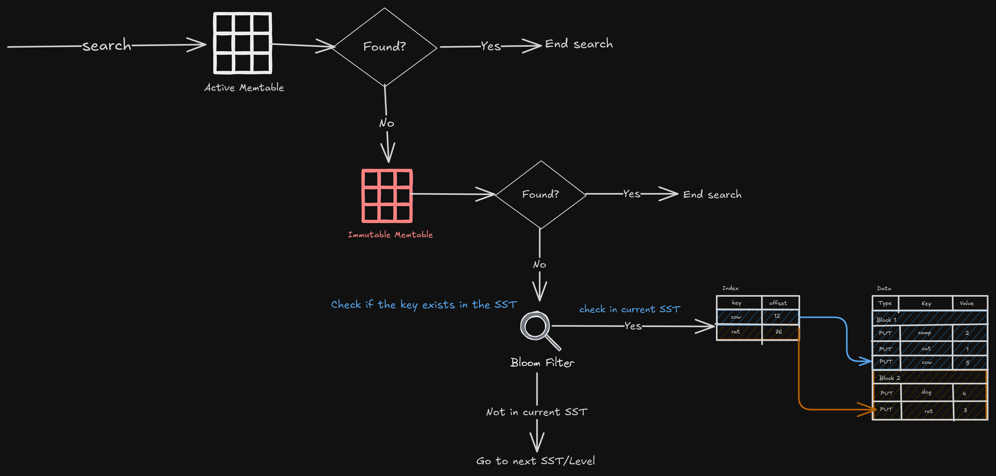
Search the active memtable
Search the immutable memtable
Go to all the SSTs, from L0 to LN, but we don’t have to search in the entire SST; we can use the bloom filter (which tells us if a key is present in the set)
If the bloom filter says it’s present, just search for the key in SST. The search is done by looking at the index offset and doing a binary search on the data.
Depending on the key, a lookup may end early at any step.
Wrapping Up
So we looked at B+ Trees and LSM Trees. Both do the same thing, but in an entirely different way. One is optimized for reads, the other for writes.
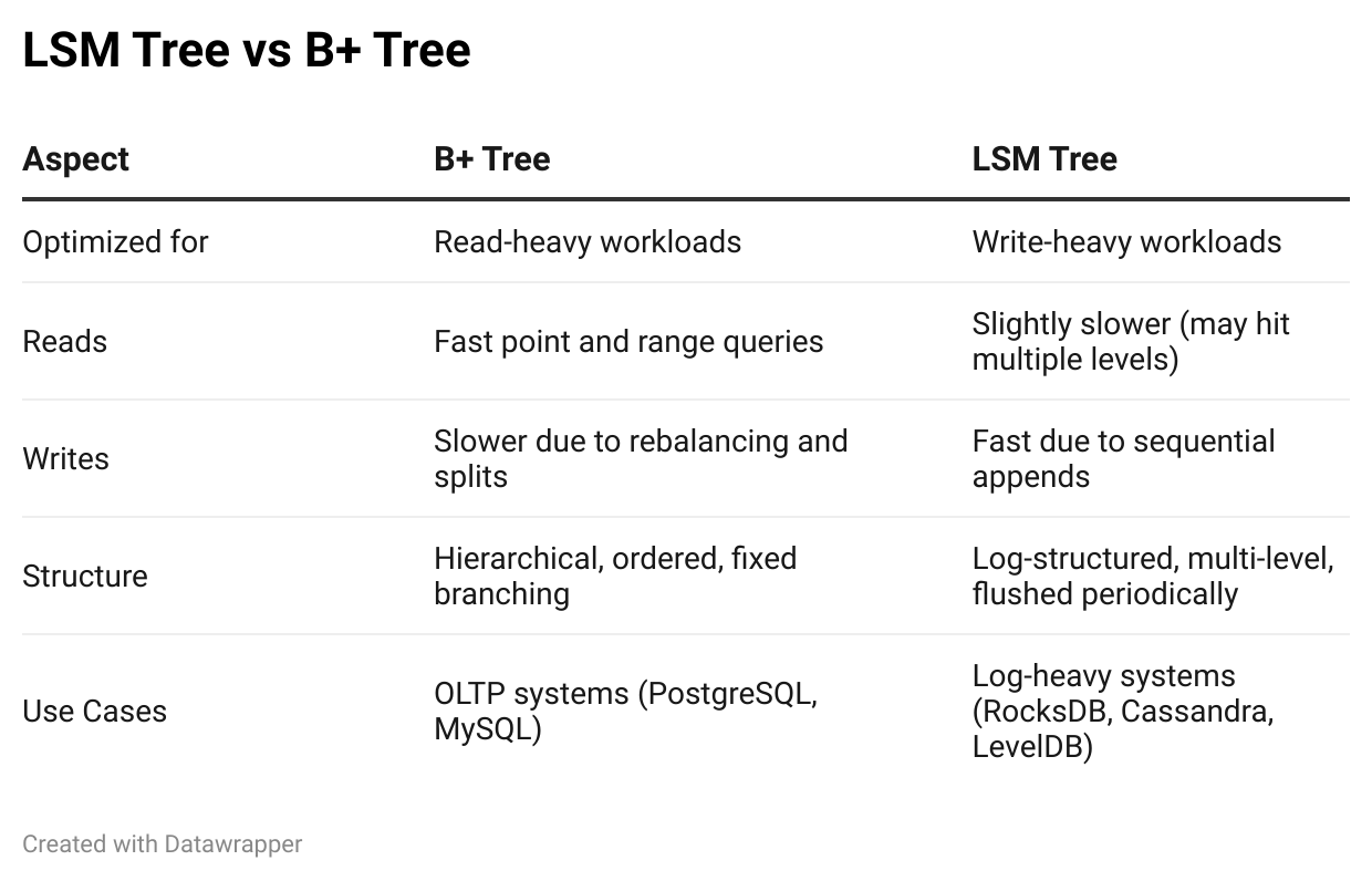
B+ Trees shine when fast lookups and range scans are the priority, which is why they’re great for traditional RDBMS systems. But when we’re handling massive writes, like in time-series databases, key-value stores, or real-time analytics engines, LSM Trees dominate with their write-friendly design.
Ultimately, we see it again, it’s all about trade-offs; there’s no "better" structure, only the right one for the job.
Understanding how these indexes behave under different workloads helps us make smarter architectural decisions, whether we’re tuning an existing system or designing one from scratch.
That’s all for this one.
Next week, I’ll be publishing the first edition of the series Breaking Prod — a deep dive into how Facebook built their Shard Manager, which handles all the painful operations of sharding at scale.
It’s been one of the hardest things I’ve studied so far. And probably the most fun.
Stay tuned!