

How Vector Databases Actually Work
Finding shortest distance in 1000 dimensions

Vector databases are what power the context in modern LLMs, and it feels magical.
Like, how does an algorithm know what I'm talking about? Am I describing something related to a cat, a dog, or a human? How can it understand the emotion of my text like another human?
It feels magical, but when we strip down the underlying mechanism, we will realize that we didn’t wake up and find vector databases one day. It was a gradual step-by-step realization, starting from just a basic database query.
Range Queries in 1 Dimension
What happens when you query an integer value in a database? Let’s assume –
WHERE amount >= 30 and amount <= 100
Relational databases do this via B+ Trees, and if you don’t know what B+ Trees are, well… I’d highly recommend you read this before you read any further.
The basic idea behind the B+ tree is that, at each node, we divide the space into two halves – a left and a right one.
The left one has all the values less than the root, and the right half has all the values greater than the root.

In theory, that’s how a B+ tree works. And if you paid close attention to the dividing into two halves aspect of B+ trees, you might realize that it is the reason for its efficiency; we’re effectively reducing our search space in half at every single node.
Now, that’s what happens when we want to do a range query in 1 Dimension.
Range Queries in 2 Dimensions
Now, the obvious question: what happens if we try to apply the same logic in 2 dimensions?
Let’s assume we have a coordinate, some latitude, longitude, say, a food-delivering app has those for a restaurant. Now, the algorithm wants to get all the free riders within a 2 km radius of this restaurant so it can assign the order to someone.
How do databases do that?
Imagine going through the entire collection of data in the table, each available rider having its own latitude, longitude, and then figuring out the math if that person is within the 2km radius, computing the entire bla bla bullshit.
Too slow.
Can we use a B+ Tree?
Hmm, let’s think it through. What happens in a B+ Tree, each node contains one value, and we decide to go left/right based on that value.
If we encode just the latitude, in each of those nodes, we would be able to at least go left/right based on the latitude of the node, but we would be running blind on the longitude, since we don’t know if all the nodes in the left/right have a longitude greater/smaller than the current one.
So, this makes us realize that 1 dimensional tree is not sufficient. We need to not just divide the surface into left/right, but also need a top and a bottom.
And well… my friends, we’re entering the territory of QuadTrees.
QuadTrees
Yes, as the name suggests, Quad – meaning 4, Trees, well… the green things that grow tall.
As in a B+ tree, every insertion is based on whether it falls to the left/right of a node; we do something similar in a QuadTree (but instead of 2, we divide the surface into 4).
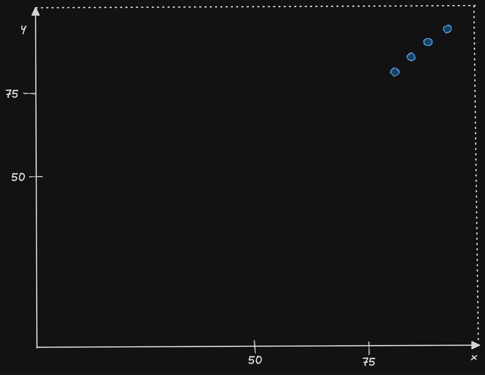
At the start, QuadTree will have a surface, assuming a 100 x 100 surface. Nothing on it right now.
Let’s insert some points, (80,80), (85,85), (90,90), (95,95)
This is what our surface looks like now –
Let’s recall how the insertion happens in a B+ tree, which will give us insights into how similar QuadTrees are.
Every B+ tree has a capacity – the maximum number of child nodes a parent can have. Once it exceeds that, the tree rebalancing happens, something like the following –
You start inserting numbers: 10, 20, 30, 40. The node is now full. It has reached its capacity of 4.
[ 10 | 20 | 30 | 40 ] <-- Node is at max capacity!Now, you try to insert 25. The node cannot hold 5 items. It must split. To split, the B+ Tree looks at the values of the data:
It sorts them: 10, 20, 25, 30, 40.
It picks the middle value (25) to push up to a parent layer.
It splits the remaining data right down the middle into two new nodes.
            [ 25 ]
           /     \
  [ 10 | 20 ]    [ 30 | 40 ]
Now, let’s look at our quad tree. Let’s imagine the capacity to be 4.
Since our surface already has 5 points, more than capacity, how do we rebalance the surface?
We draw lines at X=50 and Y=50. It creates 4 new child boxes and pushes the data down into them.
And now, the surface looks like this.
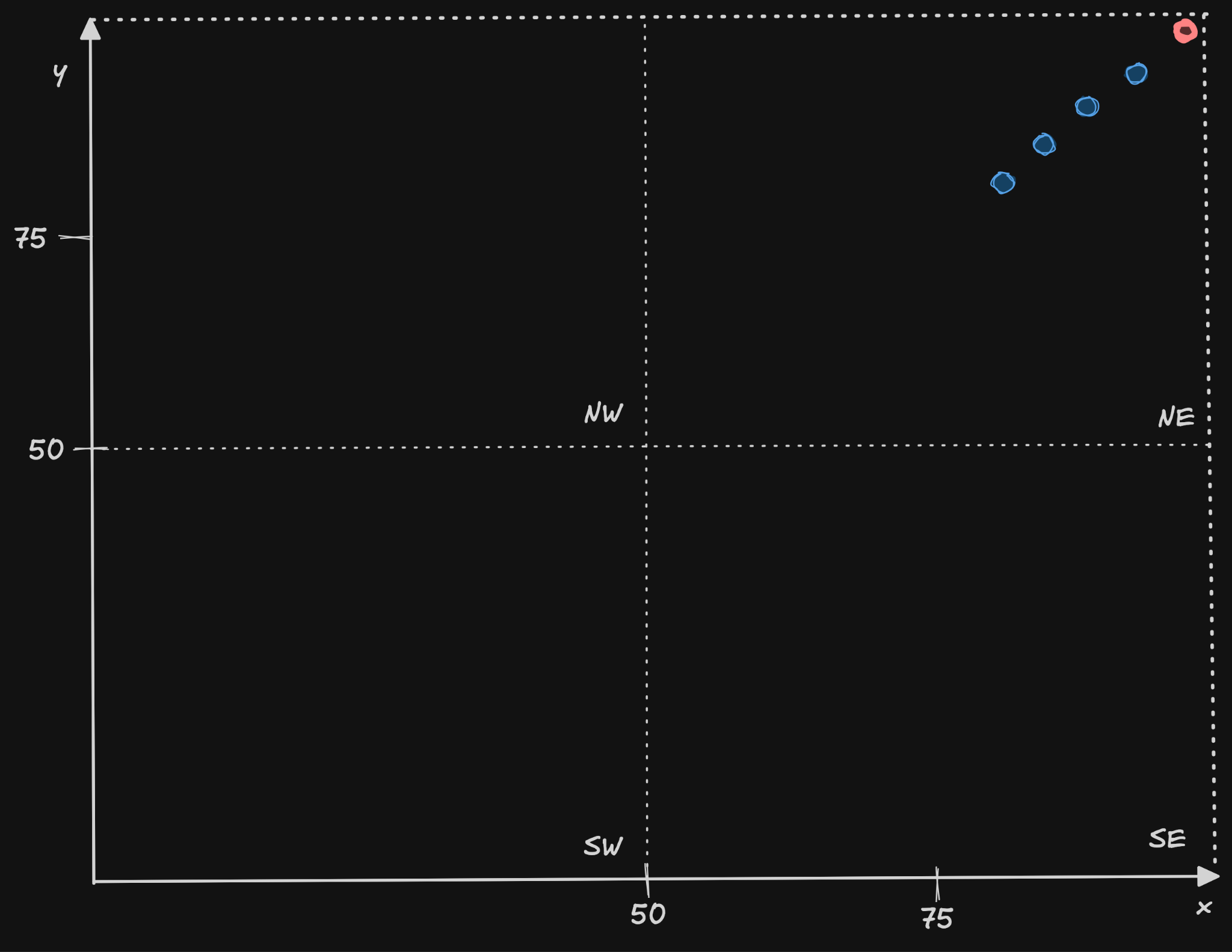
Because we blindly split the space in the middle, the NE box instantly inherits all 5 points. It is still over capacity.
So the Quadtree immediately has to split that NE box again into 4 even smaller squares (75 to 100), and it keeps doing this until no single box holds more than 4 points.
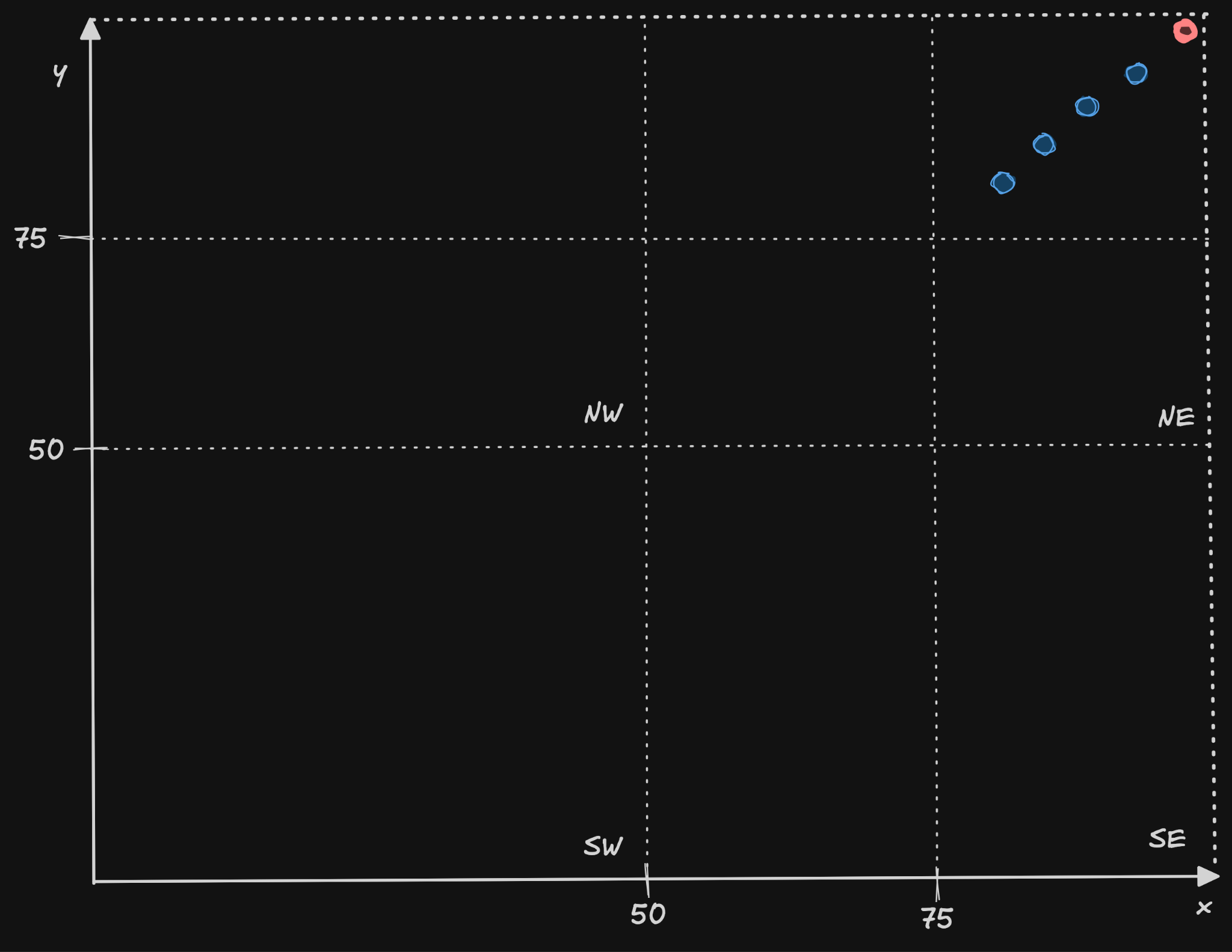
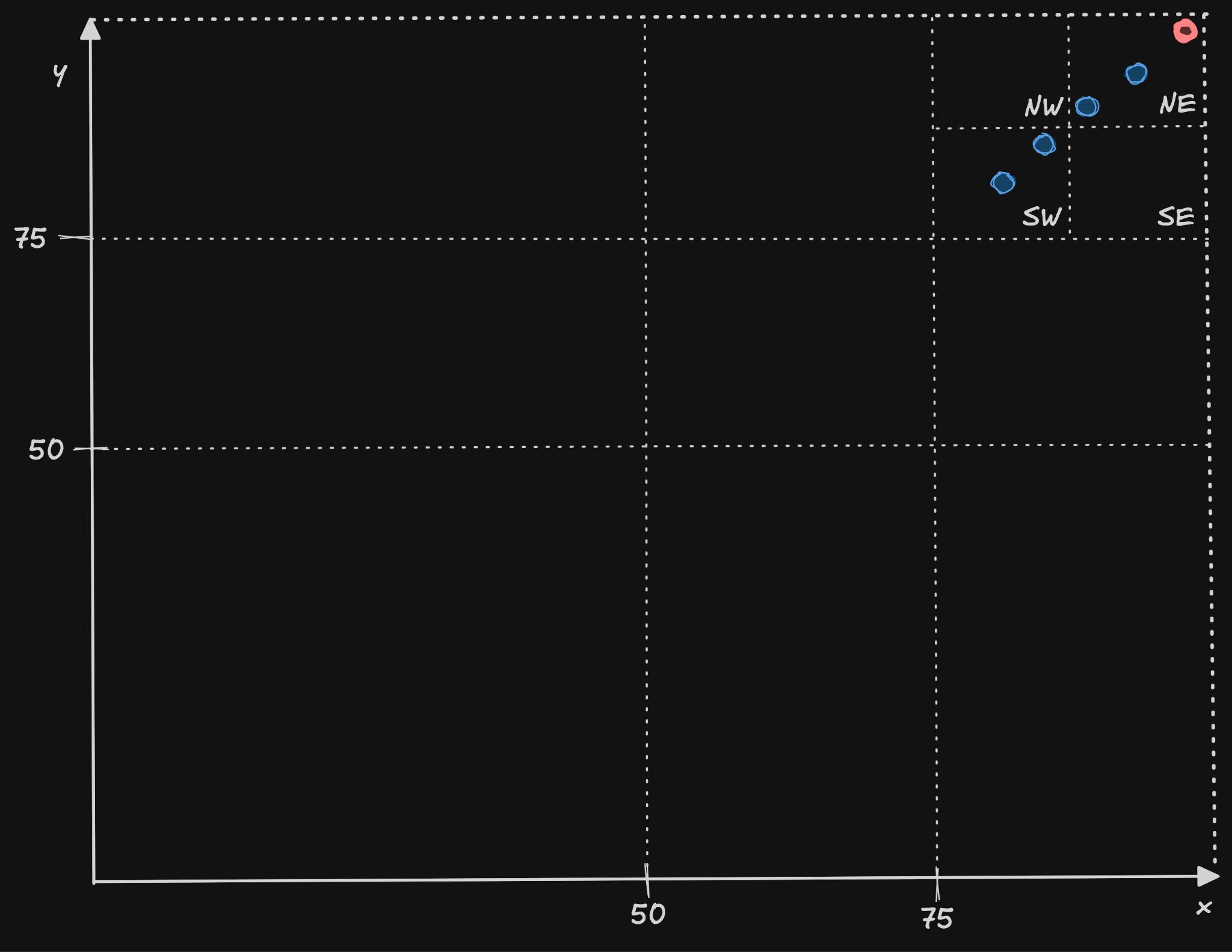
Because the Quadtree splits based on where the center is, rather than the data’s median point (as in the B+ tree), it can lead to heavy asymmetry:
Dense Clusters: If you have 1000 points crammed into a tiny 1-meter square in Mumbai, the Quadtree will have to split dozens of times recursively to isolate those points into boxes that hold fewer than 4 points each. This creates a very deep tree branch.
Sparse Wastelands: If you have 0 points in the middle of the Indian Ocean, that quadrant remains a single, giant, empty box that never splits.
Now, some of you must ask, “But why? Why are we dividing in the middle blindly?”
Because It’s Fast and Easier to Calculate Distance
Calculating boundaries by dividing by 2 is incredibly fast.
In fact, at the hardware/CPU level, dividing an integer or a floating-point number by 2 can often be optimized to a simple bit-shift operation or basic subtraction.
If the parent box is (0,0) to (100,100), the center is obviously (50,50). The database engine doesn’t have to think, analyze, or run any complex statistical math; it just cuts the space in half and moves on.
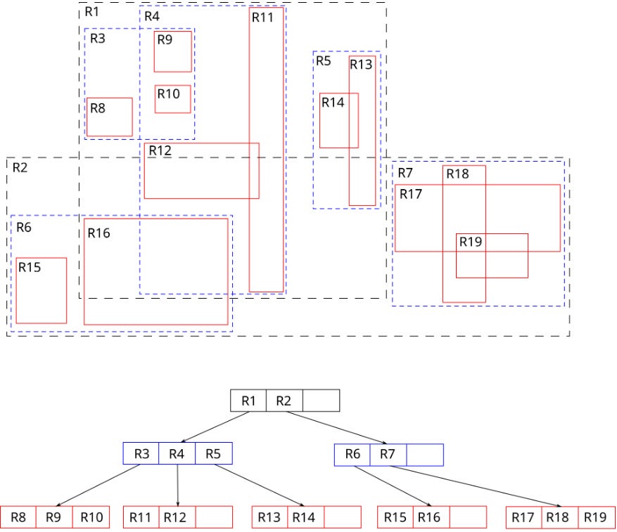
But production geospatial databases (like PostGIS in PostgreSQL) rarely use pure Quadtrees. Instead, they use R-Trees (Rectangle Trees).
R-Trees are even more complex versions of QuadTrees; they can also work in 3 Dimensional space. The idea behind R-Tree is simple —
When an R-Tree node reaches capacity:
It looks at the cluster of points.
It finds a way to divide those points into two groups such that the total area of the two new wrapping rectangles is as small and tight as possible.
The bounding boxes are allowed to overlap, and their shapes change dynamically based on the data.
I found a good illustration of R-Tree from Wikipedia —
If we extend R-Tree to 3D, this is what we get —
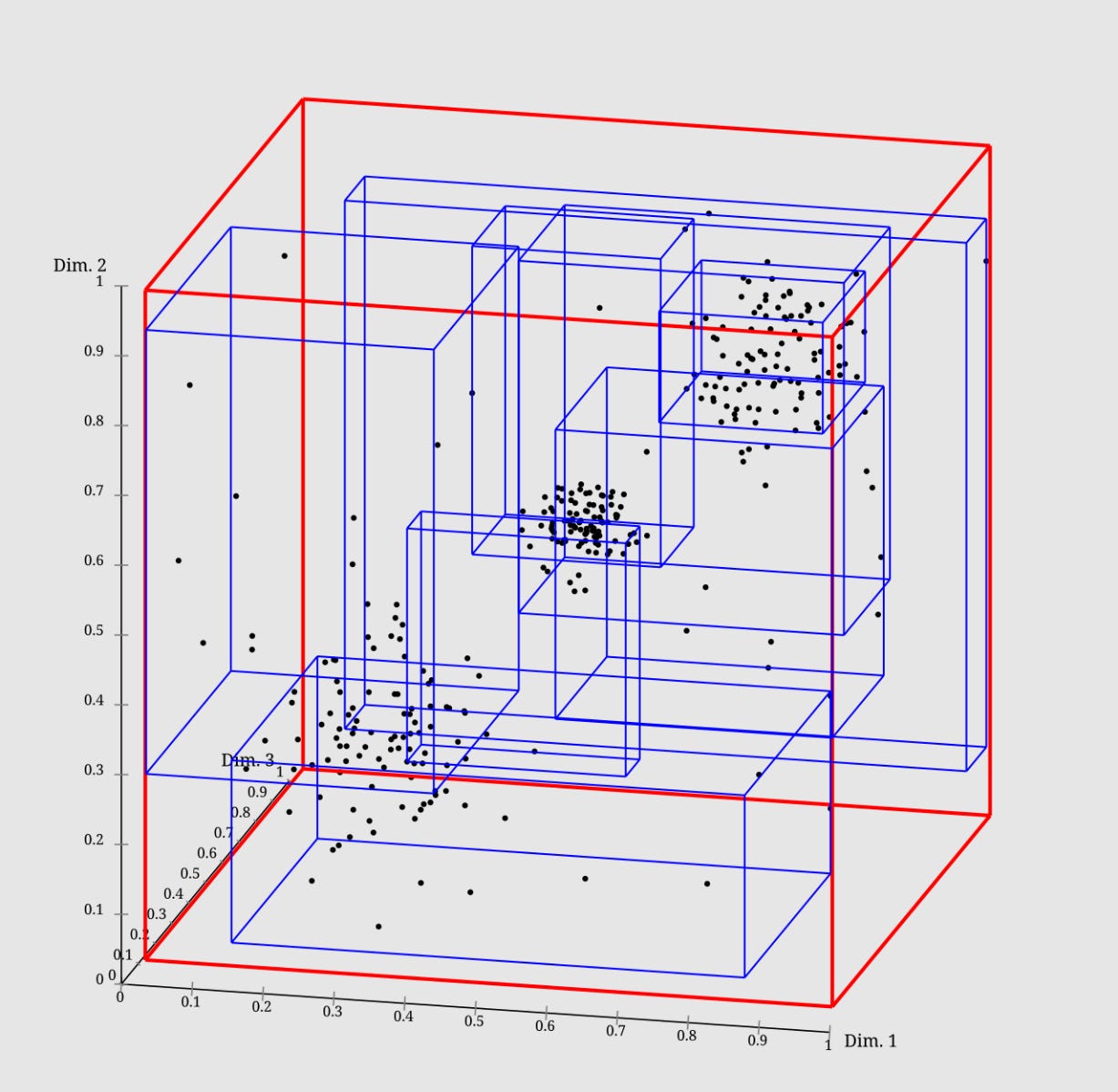
So, till now, we have understood how a range query works in 2 dimensions. If we extend the same idea in 3 dimensions, we will be working with OctaTree (each node having 8 neighbors).
OctaTree can be used in game engines to compute distances in 3D spaces.
Now that we are acquainted with the 3-dimensional “nearest neighbor” problem, let’s move to higher dimensions.
Range Queries in N Dimensions
Can we extend the idea of OctaTree to something like n(something)Tree?
Let’s try.
But before we even touch on how to query in n-dimensional space, we need to understand how things look in more than 3 dimensions, because we’re a 3D creature; it’s not trivial to imagine higher-dimensional objects the same way.
Most n-dimensional objects can be called a “vector” – an arrow pointing to a coordinate in n-dimensional space.
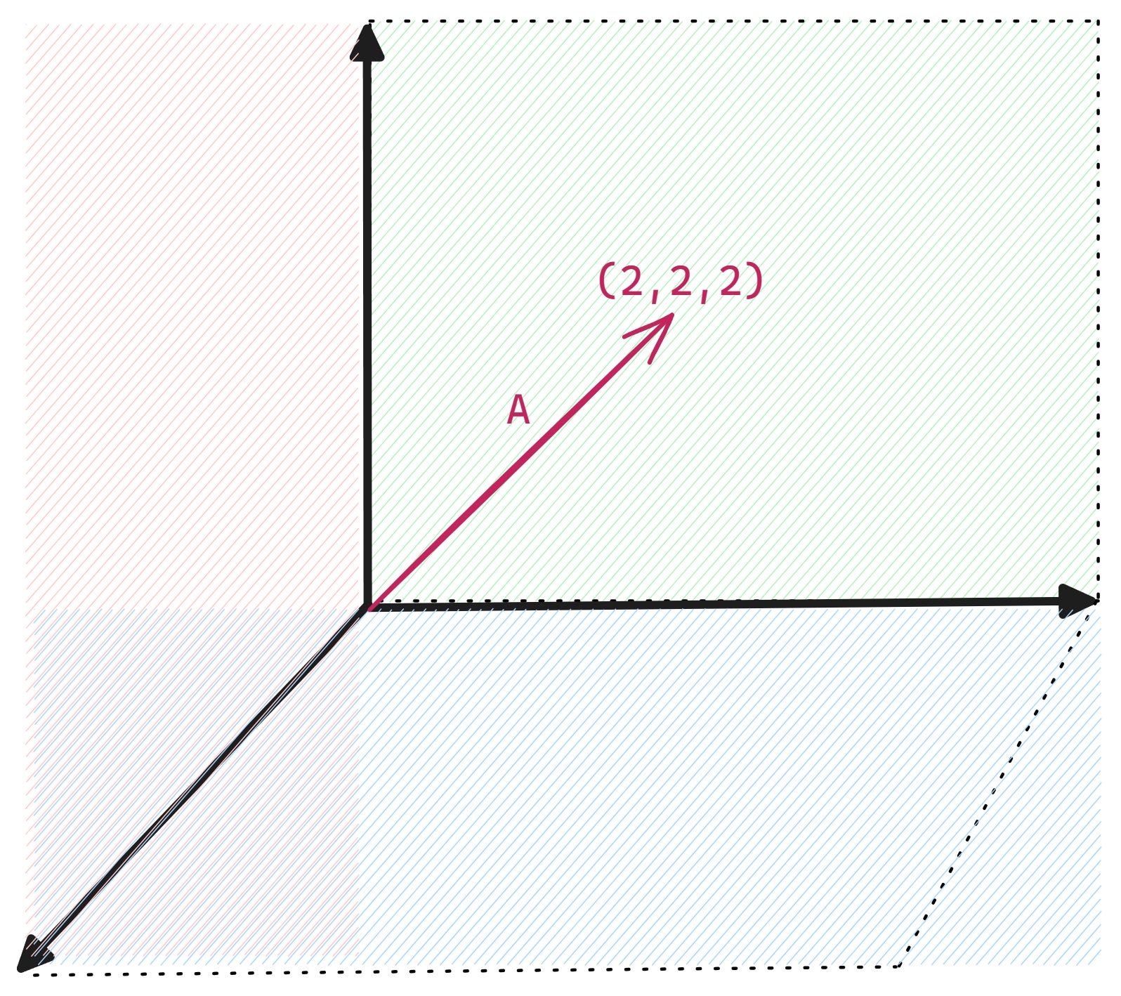
But I always found that a bit hard to visualize, so instead of visualizing it, let’s treat a vector as a detailed profile or a feature checklist.
Let’s say we want to represent Houses as vectors.
1D Vector (A single line)
Features: [ Size in sq ft ]
Example: [ 2500 ]
Visualization: A single point on a ruler. Easy.
3D Vector (A physical room)
Features: [ Size, Number of Bedrooms, Price ]
Example: [ 2500, 3, 500000 ]
Visualization: You can map this on an X, Y, Z graph.
6D Vector (nD)
Now, let’s add more features. We want to capture: [ Size, Bedrooms, Price, Distance to metro (km), Age of building, Crime rate index ].
Example House A: [ 2500, 3, 500000, 0.5, 5, 12 ]
Example House B: [ 2400, 3, 490000, 0.6, 6, 11 ]
Of course, you cannot draw a 6D graph on paper.
But if you look at the two arrays above, the brain instantly recognizes that House A and House B are extremely similar. They are basically identical twins in terms of their profile.
That is all an n-dimensional vector is. It’s just a list of n quantitative metrics describing an object.
When a vector database calculates “distance” between two 1000-dimensional vectors, it isn’t just moving an arrow through hyperspace (it does so mathematically); it’s also comparing two massive checklists to see how much their numbers align.
Distances in Space
If you recall what you learnt in maths (yes, those formulas do matter), the Euclidean (straight-line) distance between 2 points in a 2D space is –
Extending this to a 3D space is as simple as –
And the beautiful thing about this formula is that it works the same for even a 100-dimensional –
When an AI embedding model looks at text or an image, it translates abstract human concepts into these n-dimensional arrays.
Let’s imagine a 4-dimensional text embedding model where the dimensions secretly represent: [ Is it an animal?, Is it royal?, Is it male?, Is it a tool? ]
“King” might look like: [ 0.01, 0.99, 0.95, 0.00 ] (Not an animal, highly royal, highly male, not a tool)
“Queen” might look like: [ 0.01, 0.99, 0.02, 0.00 ] (Not an animal, highly royal, NOT male, not a tool)
“Hammer” might look like: [ 0.00, 0.00, 0.50, 0.98 ] (Not animal, not royal, gender-neutral, highly a tool)
If you run the distance formula between “King” and “Queen”, the math says that there’s a tiny distance because their lists match almost perfectly except for the “male” slot.
If you compare “King” to “Hammer”, the distance is massive.
But in reality, AI models use 1,536 or 3,072 dimensions. We don’t know exactly what feature each dimension represents because the AI figured them out on its own, but the underlying principle is the same.
Now that you have the lens to see nD as just a long array of numbers, let’s tie it back to our previous topic.
If we recall, a Quadtree (22 = 4 children) and an Octree (23 = 8 children) split the space exactly in the middle?
And if we try to build a midpoint-splitting tree for a 100-dimensional vector space, a single split would require — 2100 nodes
That number 2100 is roughly around 1.26 x 1030. That is more than the estimated number of liters of water on Earth.
A single-node division would instantly crash any computer’s memory.
And this is why a normal spatial tree doesn’t work at such higher dimensions.
We needed something else to solve the same problem that we did easily in a lower dimension — “how to find the nearest neighbor in higher dimensions?”
Social Network Graph
There’s an excellent video on this from Veritasium, and I remembered it while writing this article.
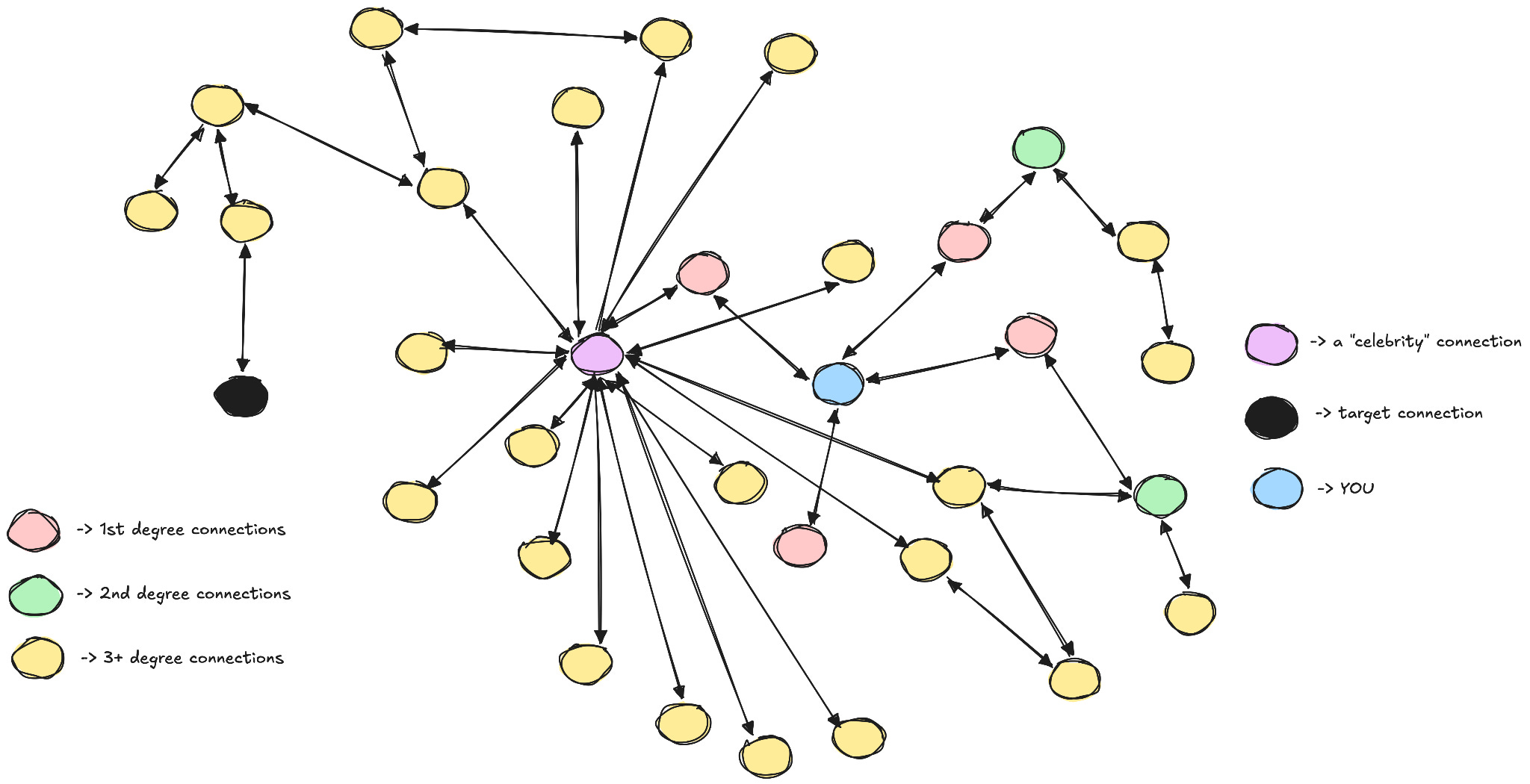
The concept states a really weird but fascinating observation about how humans are connected –
Every human on Earth is connected by at max ‘n’ degrees of separation.
If we want to contact a person, we obviously don’t have a global map of every person on Earth with their coordinates; instead, we have these connections.
If you want to pass a message to a random software engineer in Kenya, you don’t have to search all 8 billion people sequentially.
You might ask your friend who works at a global tech company.
They introduce you to their colleague in London.
That colleague knows someone managing a remote team in East Africa.
And… you’ve reached your destination in 4 jumps.
This works because human society is a Small World Network. It has two distinct types of connections:
Local Clusters: You have a close circle of friends who all know each other (high clustering).
Global Hubs: You or your friends know a few people who live far away, act as bridges to completely different social circles, or travel frequently.
Transforming Vectors Into a Social Network Graph
But how do we transform these mathematical constructs (vectors) into something that can simulate human connections?
Well, instead of thinking of vectors as being drawn on a 1000-dimensional space, let’s think of it as a person living on that coordinate.
When we insert a vector, the database connects it to its “nearest neighbors” with explicit edges, turning the database into a massive graph.
Now, to find the nearest neighbor of a vector, we just follow the nodes and compare distances until we can’t find any nodes closer.
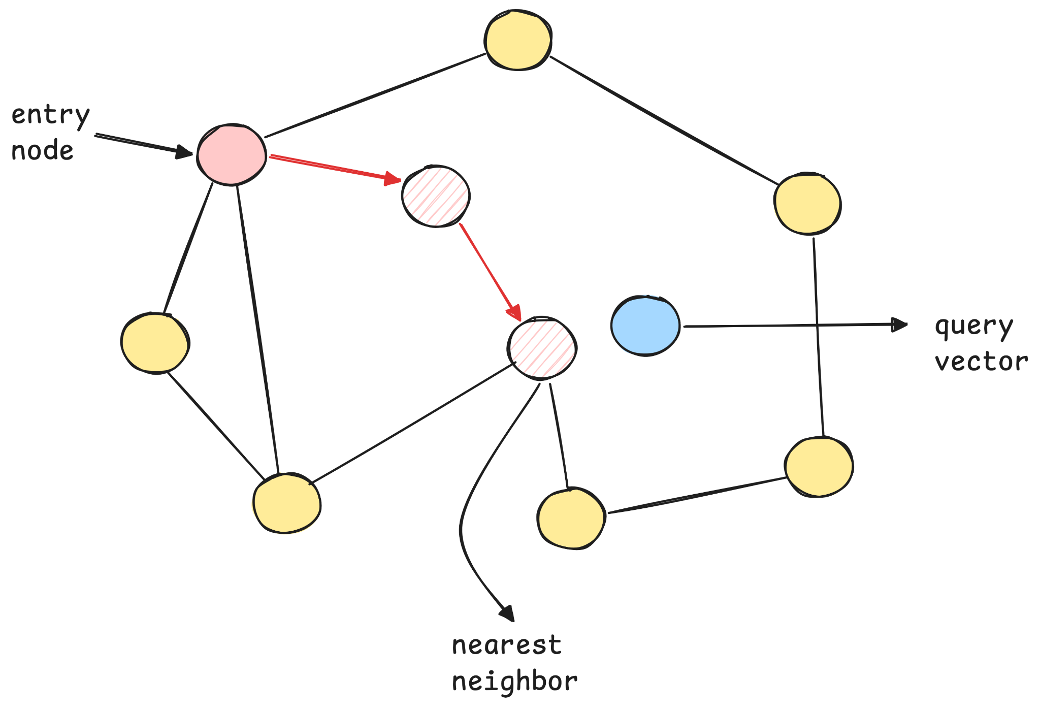
But if we build one massive graph of interconnectivity between people, it would be extremely difficult to find a node from one side of the graph to another. We would have to crawl through all the nearest neighbors of that closed-knit space for each node (for people with an algorithm background, it would be something similar to BFS, just in hyperspace).
To fix this bottleneck, an algorithm called Hierarchical Navigable Small World (HNSW) was designed (I hate its name).
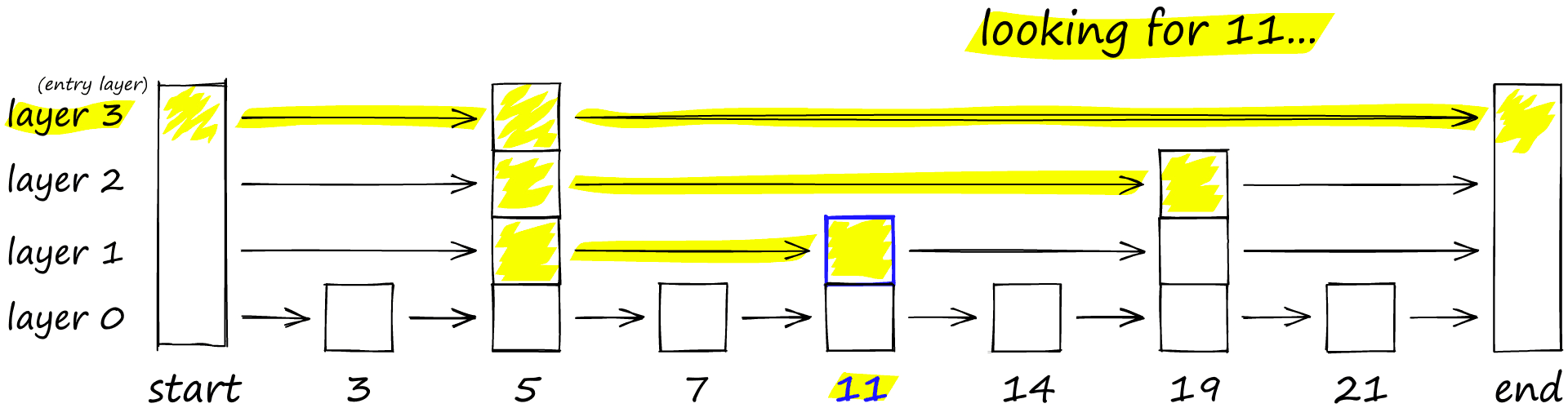
HNSW introduces a hierarchical multi-layered graph, something like a skip-list.
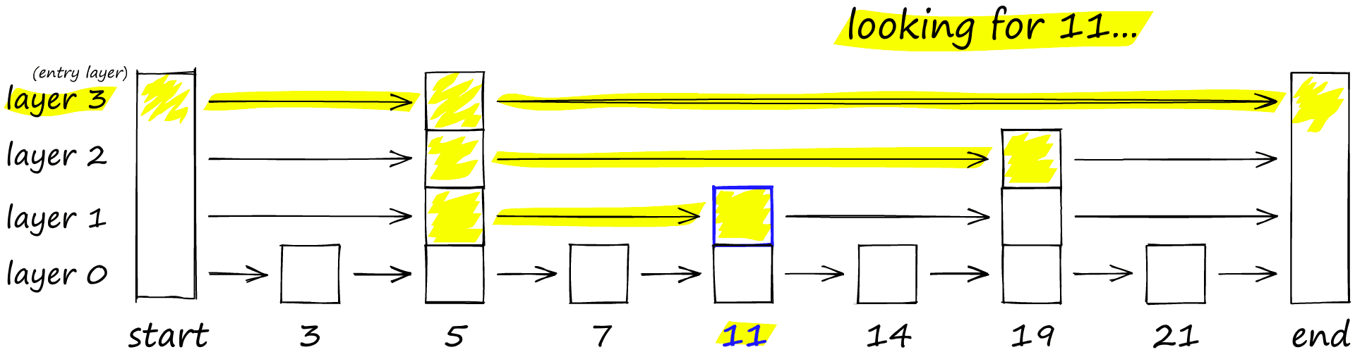
Because these are all just mathematical constructs, I’ll be simplifying them, but the underlying mechanism remains the same.
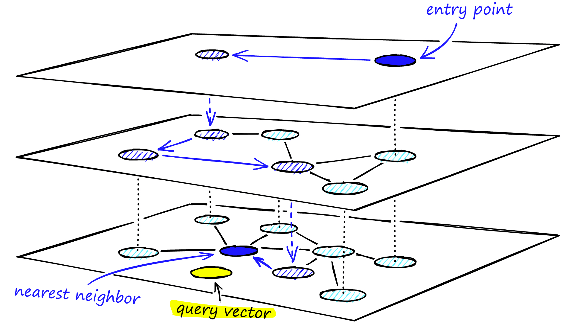
Let’s understand how a search operation happens in this space.
Layer 2 – The Airplane Layer
This layer contains only a tiny fraction of your vectors (the “global hubs”).
The connections here span massive distances across the 1000D space.
The Search: When a query comes in, the database starts at a random node on this top layer. It takes massive, sweeping jumps across the space to quickly get into the correct general timezone/continent of your query. Once it can’t find any closer nodes on this layer, it drops down a level.
Layer 1 – The Highway Layer
This layer contains a few more vectors. The connections are shorter, bridging cities or neighborhoods.
The Search: The database picks up exactly where it dropped off from Layer 2. It zooms in closer to the target vector, hopping between regional nodes until it can’t get any closer. Then, it drops down to the final layer.
Layer 0 – The Local Streets
This layer contains all of your vectors. Every single data point is mapped here with its absolute closest semantic neighbors.
The Search: The database lands right in the exact neighborhood of your target. It does a quick, short crawl through the immediate local connections to find the exact nearest matching vectors.
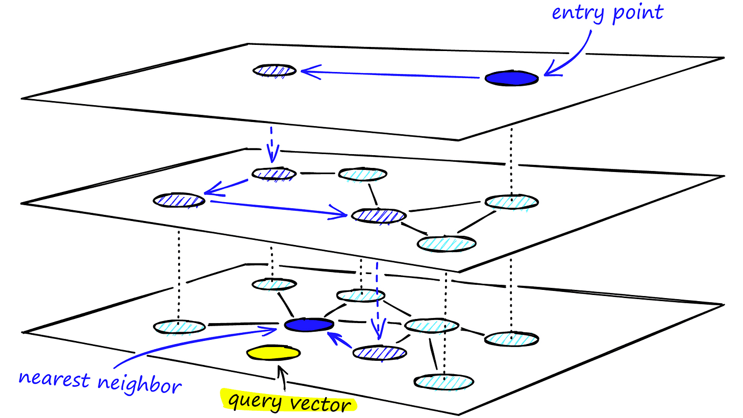
Layered graph of HNSW, the top layer is our entry point and contains only the longest links. As we move down the layers, the link lengths become shorter and more numerous — Credits
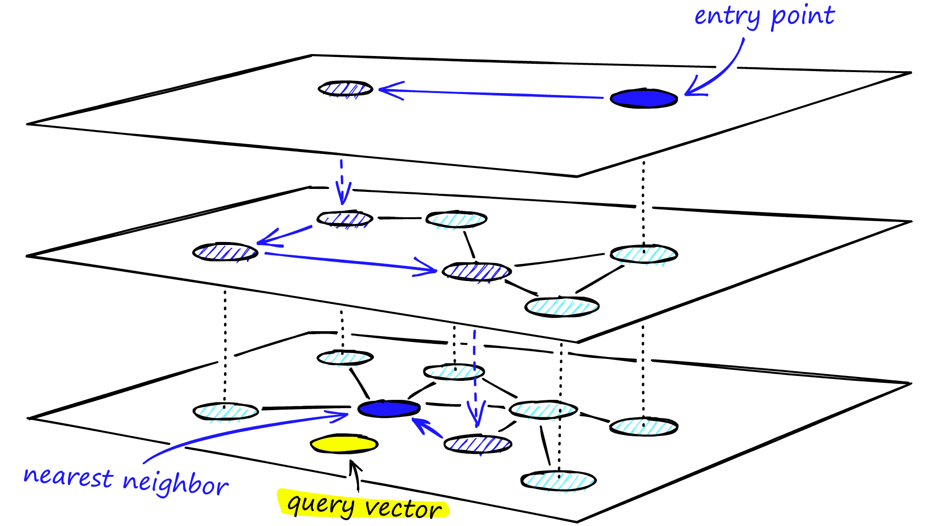

When I first found this algorithm, it was fascinating, the way we can reason about these hyperspace constructs by using just some human terms… It’s absolutely worth the awe.
If we compare it to our lower-dimensional Quad/Octa Tree –
No Spatial Explosion: The database never creates 2100 empty boxes. If you have 10000 vectors, you have exactly 10000 nodes in your graph, plus a few duplicate hub nodes on upper layers. Space is completely determined by where the data actually exists.
Amazing Speed: Because you can use the top layers to skip over massive expanses of irrelevant data instantly, the time it takes to find your nearest neighbor scales logarithmically, O(log N)—even if your vectors have thousands of dimensions
Okay, fine, search makes sense, but how do we even insert a node in this massive, weird graph?
Insertion in HNSW
Let’s try to insert a brand new vector in this database. Let’s call it a node.
Step 1 – Assigning a Random Max Layer
Since probability goes downwards layer by layer. 100% of nodes get inserted into Layer 0 (the local streets). Roughly 10% make it to Layer 1, 1% to Layer 2, and so on.
We get a random number between 0 and 1. Let’s say our New Node gets lucky and its max layer is determined to be Layer 1 (the highway layer). This means it will exist on both Layer 0 and Layer 1.
Step 2 – Downward Search (Finding the neighbors)
The database enters the graph at the top-most layer, Layer 2 (the Airplane Layer), at a default entry point.
On Layer 2, it performs a quick search to find the node that is closest to our New Node.
Once it finds that closest node, it drops down to Layer 1 at that same coordinate.
Step 3 – Inserting into Different Layers
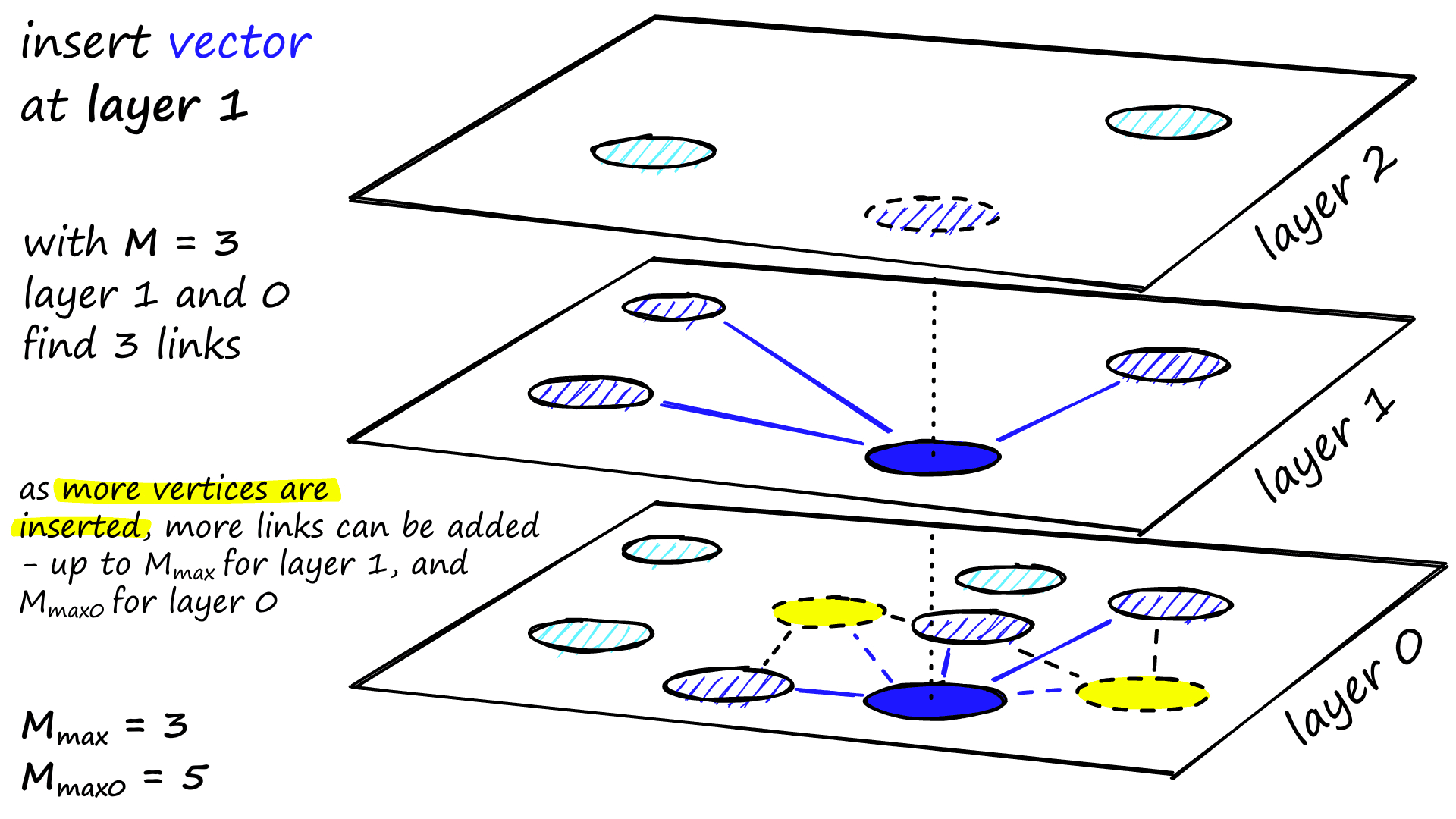
Now that the database has dropped down to Layer 1 (Highway Layer, the maximum layer assigned to our New Node), the real insertion work starts –
Find the M Closest Friends: On Layer 1, the database searches for the absolute closest neighbors to our New Node. The database has a configurable parameter called M (e.g., M=4), which is the maximum number of connections any node can have at a particular level. It finds the top M closest neighbors.
Bi-directional Linking: The database places the New Node onto Layer 1 and draws lines (edges) connecting it to those M neighbors. These connections are bi-directional. The neighbors now point to the New Node, and the New Node points to them (so that we can reach both of them vice versa).
Drop and Repeat: The database drops down to Layer 0, takes the closest points it found from Layer 1 as its starting point, searches for the closest M neighbors on the crowded local streets, and connects itself to them as well.
If you pay close attention to the algorithm above, you might find that there’s a huge problem with this approach.
What if a few nodes are really popular? They might be connected to a lot of neighbors, making them highly inefficient to narrow down our searches to lower layers.
To prevent this, HNSW runs a pruning algorithm during insertion (you can draw the similarities of rebalancing of B+ Trees, or rearranging the points after division of the surface in a QuadTree).
Pruning of Neighbors
If adding the New Node causes an existing node to exceed its limit of M connections, that old node is forced to re-evaluate its friends:
It looks at its M+1 connections.
It measures the distance to all of them.
It keeps the closest/most structurally diverse ones and breaks the connection with the furthest one.
This keeps the density of the entire network uniform and bounded, ensuring that no single node ever becomes a bottleneck.
We have essentially built the algorithm that most vector databases use internally to understand the context before giving it to an LLM.
If you ask me, I think this might be the coolest algorithm I’ve read in the last few years.
How it Connects to RAG (Retrieval Augmentation Generation)
The algorithm we just figured out is the R (Retrieval) part of the RAG.
It is essential to know how to find useful contexts in a huge ocean of interlinked information.
You could try to do RAG without a vector database by just stuffing every file you own into the LLM prompt every single time. But LLM prompts have strict context windows, and passing millions of words to an LLM for a simple question is highly expensive and absolutely slow.
The vector database acts as the intelligent filter. It reduces gigabytes or terabytes of corporate knowledge down to the exact 3 or 4 paragraphs needed to answer a specific question in under 50 milliseconds.
Closing Thoughts
We went from 1-dimensional nearest neighbor to finding nearest neighbors in n dimensions —
1D Space (B+ Trees): Traditional database rules apply here by splitting sorted data down the middle. It keeps searches fast O(logN) because every step drops half the remaining data keys.
2D/3D Space (Quadtrees & Octrees): The moment we add spatial dimensions (like latitude and longitude), splitting data fails. We shift to splitting geometric space into fixed, uniform quadrants. It works beautifully for maps.
The nD Explosion: When AI models translate concepts into 1536-dimensional vectors, spatial splitting breaks down entirely. Splitting a 100-dimensional space requires 2100 subdivisions, a geometric explosion that would instantly melt a computer’s memory.
HNSW (The Social Network Solution): To survive high dimensions, we completely abandon spatial grids and treat vectors like people in a Small World Network. By organizing points into explicit, layered connectivity graphs, we get a multi-layer navigational system that lets queries skip across global hubs and dive into local neighborhoods in milliseconds.
Now, I am not an ML/AI guy, and I always feel that I am late to the AI hype party that everyone keeps talking about. But the more I understand these fundamental concepts, AI doesn’t feel like magic; it’s just pure maths, amazing algorithms, and the application of absurdly powerful software engineering principles at scale.
And the culmination of everything makes the end product (AI) feel “magical.” And I don’t like magic.
This entire article started from one question: how do you find the closest point in 2D space?
But when I kept pulling that thread, extending it to 3D, then to n dimensions, I realized vector databases are not doing anything magical. They’re solving the same geometric problem you learned in 9th grade, just in 1536 dimensions.
Now you know how an algorithm understands whether you’re talking about a cat, a dog, or a human. It’s not magic. It never was.
A Message
I’m a backend engineer, not an AI philosopher. I write these posts because I believe the best way to understand complex infrastructure is to strip away the magic and look at the system architecture from absolute first principles.
If mapping B+ Trees to social networks gave you a cleaner mental model for how vector search actually functions, that’s a win for me.
If you want to support more of this, you can here. No pressure, genuinely!